Why Mathematics?
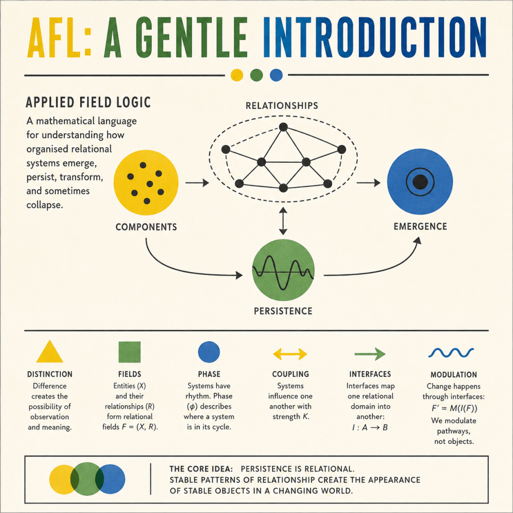
Applied Field Logic did not begin with mathematics. It began with a simple observation.
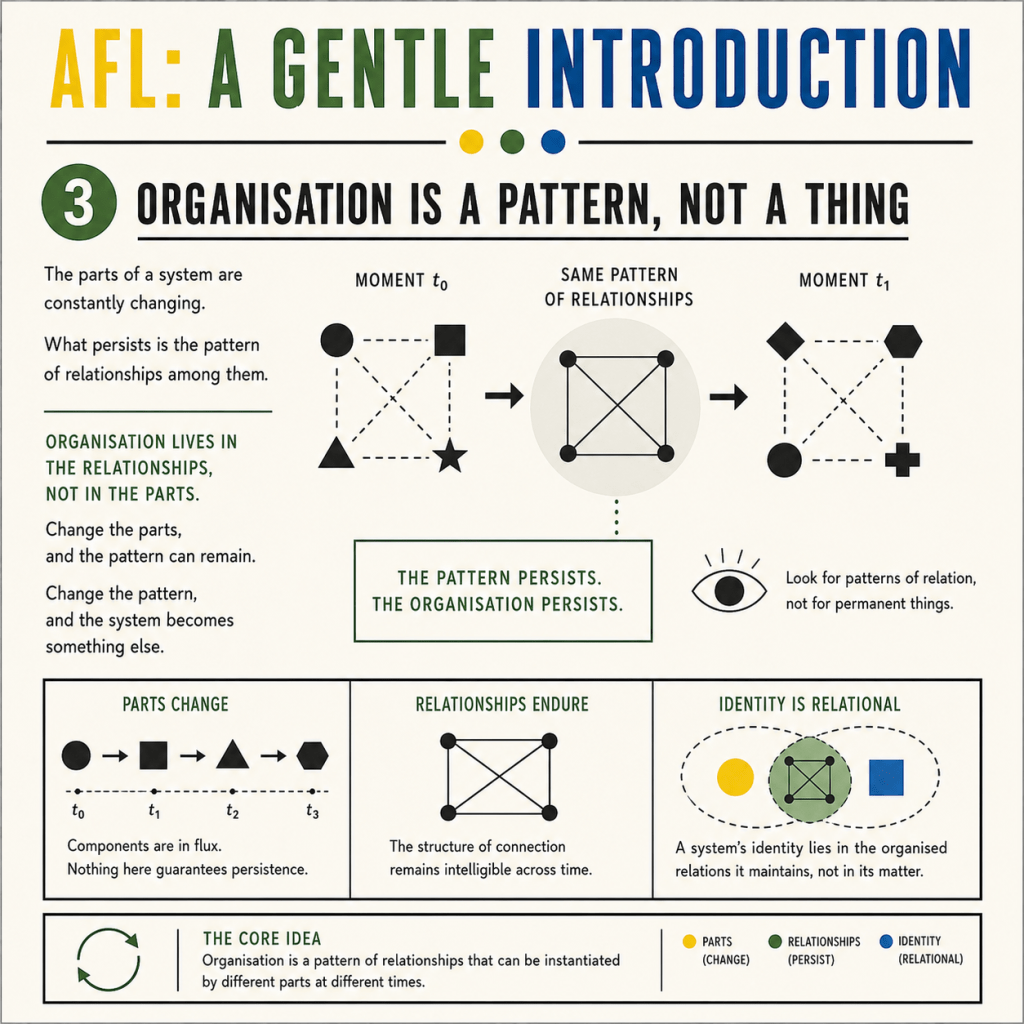
Things persist while everything inside them changes.
Your body replaces its cells. Languages replace their words. Economies replace their participants. Ecosystems replace their organisms. Yet something remains recognisably the same.
The purpose of mathematics here is not to confer authority. Mathematics is simply a language of precision. It allows ideas to be stated clearly, assumptions to be exposed, models to be constructed, and predictions to become testable.
This tutorial assumes only high-school algebra and an intuitive understanding of graphs. Every symbol is introduced before it is used. Every equation is translated back into ordinary English.
—
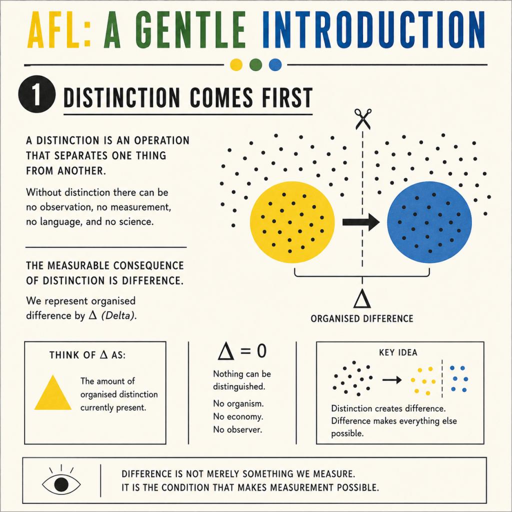
Step 1: Distinction Comes First
Classical science often begins with objects.
Applied Field Logic begins with distinctions.
A distinction is an operation that separates one thing from another.
Without distinction there can be no observation, no measurement, no language, and no science.
The measurable consequence of distinction is difference.
We represent organised difference by the Greek letter
Δ (Delta)
Think of Δ simply as:
«The amount of organised distinction currently present.»
If
Δ = 0
then nothing can be distinguished.
No organism.
No economy.
No observer.
Difference is therefore not merely something we measure. It is the condition that makes measurement possible.
—
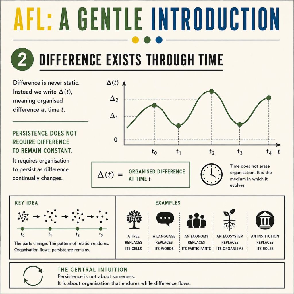
Step 2: Difference Exists Through Time
Difference is never static.
Instead we write
Δ(t)
meaning
«Organised difference at time t.»
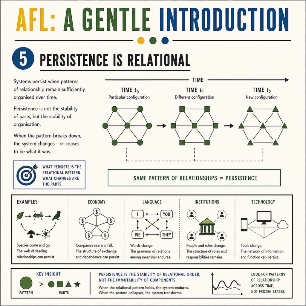
Persistence does not require difference to remain constant.
It requires organisation to persist as difference continually changes.
—
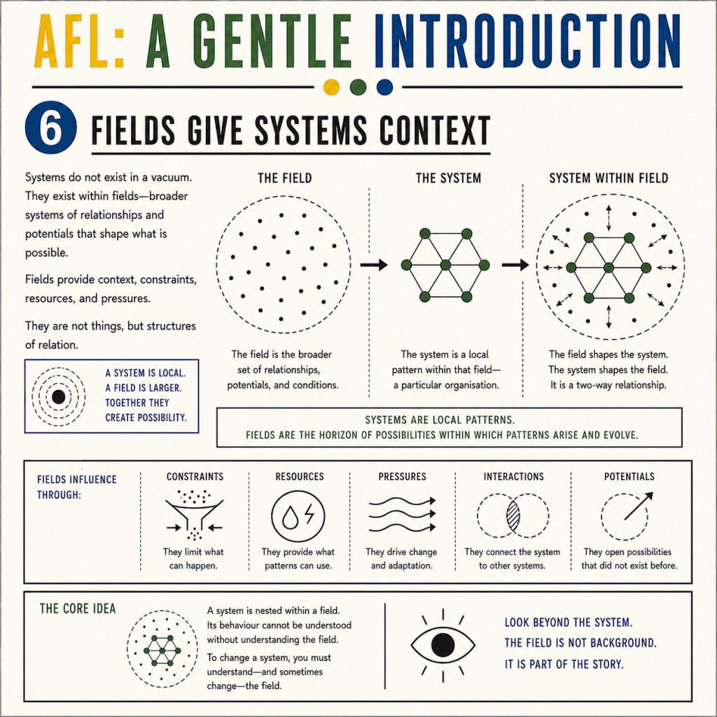
Step 3: Fields
Applied Field Logic is ultimately a theory of fields rather than isolated objects.
We define a field as
F = (X, R)
where
X represents entities,
and
R represents the relationships connecting them.
Without relationships there is no field.
A collection of disconnected objects is not yet a system.
—
Step 4: Persistence
Persistence is not a substance.
It is organised difference maintained through time.
As a first approximation we may write
P = ∫ Δ(t) dt
This should be read as a conceptual summary rather than a complete definition.
It captures the central intuition that persistence emerges from continuously maintained organisation rather than static material.
A more rigorous functional is developed in the mathematical foundations paper.
—
Step 5: Phase
Many systems possess rhythm.
Heartbeats.
Speech.
Markets.
Seasons.
Climate.
We represent timing using
φ (phi).
Phase describes where a system currently lies within its own cycle.
Applied Field Logic proposes that, in many complex systems, timing can be as important as magnitude.
Two systems may contain similar energy while behaving very differently simply because they are out of phase.
—
Step 6: Coupling
No complex system exists in isolation.
Systems influence one another.
We represent that influence by
K
the coupling strength.
Large K indicates strong interaction.
Small K indicates weak interaction.
Forest → Rainfall
Rainfall → Agriculture
Agriculture → Economy
Economy → Politics
Politics → Energy
Each connection is a pathway through which organisation propagates.
—
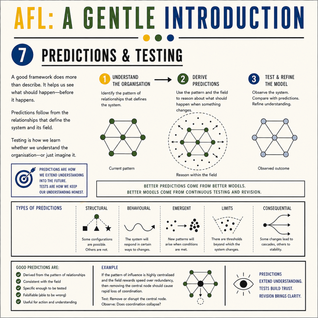
Step 7: Synchronisation
The mathematics of synchronisation is already well established.
One standard model for coupled oscillators is
dφᵢ/dt = ωᵢ + (K/N) Σⱼ sin(φⱼ − φᵢ)
The details are less important here than the underlying idea.
Each system possesses its own preferred rhythm.
Coupling allows those rhythms to influence one another.
Order emerges through interaction rather than central control.
Applied Field Logic adopts synchronisation as one mathematical language for describing organised persistence.
—
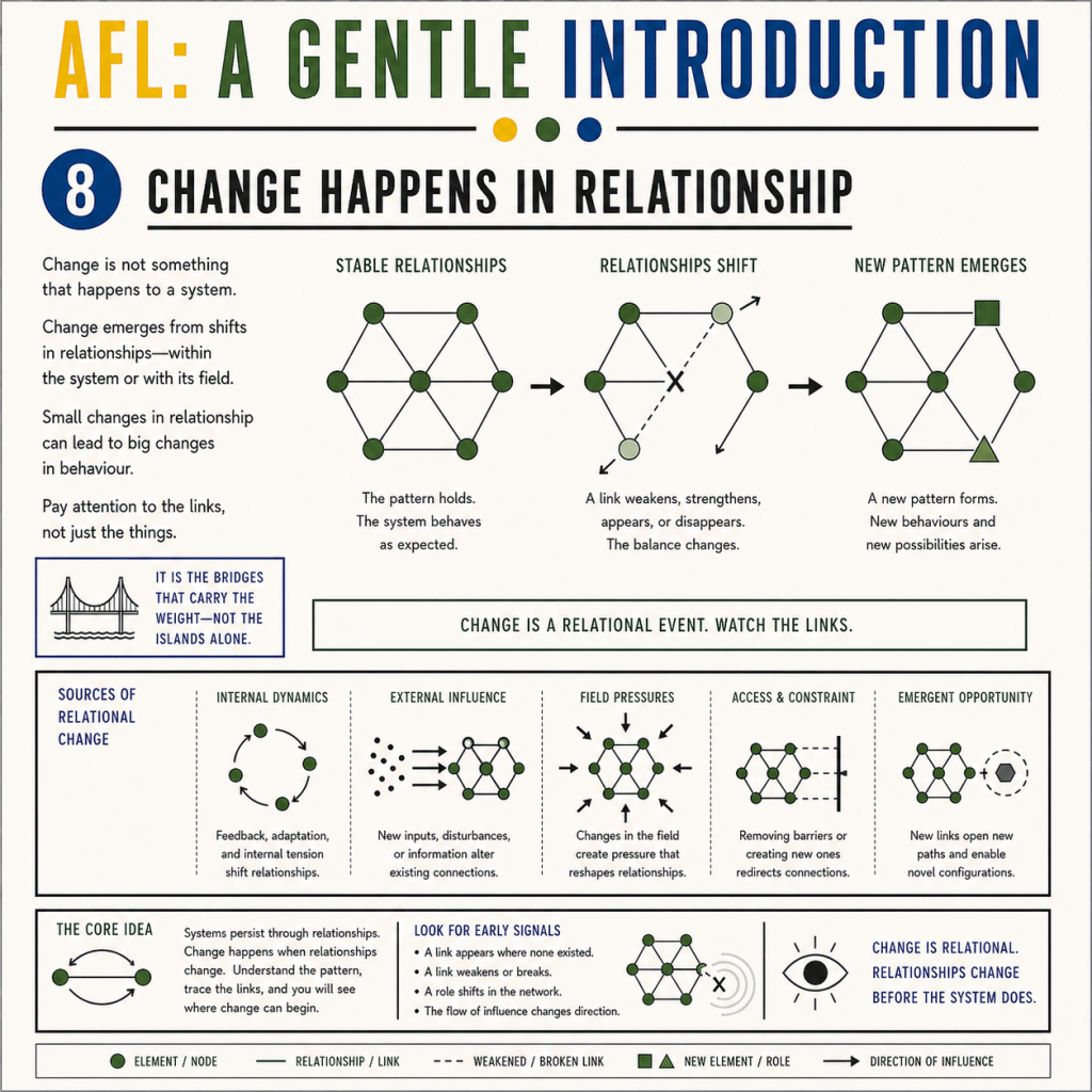
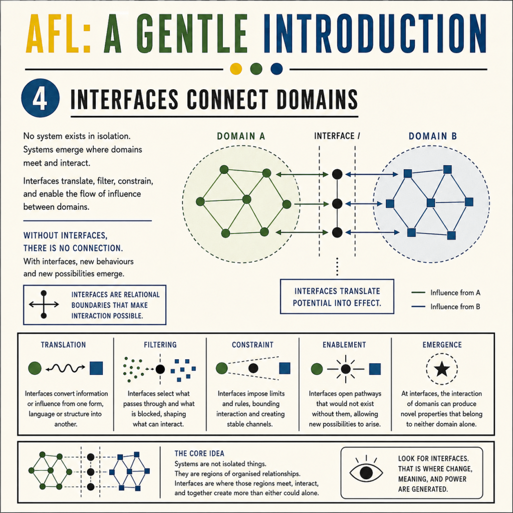
Step 8: Interfaces
Applied Field Logic introduces interfaces.
An interface maps one relational domain into another.
We write
I : A → B
meaning
«Interface I transforms relational domain A into relational domain B.»
Examples include
Human activity → Atmospheric energy
Resources → Prices
Thought → Language
Events → Public attention
Interfaces do more than connect systems.
They transform one form of organisation into another.
—
Step 9: Interface Operators
Many interfaces act not on isolated variables but on entire relational fields.
We therefore write
I(F) = F′
meaning
«Interface I transforms relational field F into a modified field F′.»
The apostrophe simply indicates that the field has been transformed.
Interfaces therefore become operators acting upon relational organisation itself.
—
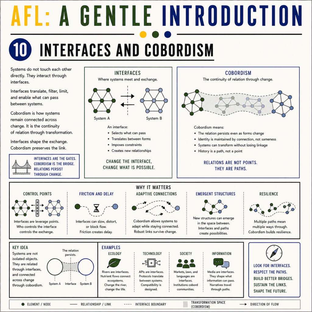
Step 10: Interfaces and Cobordism
Topology provides a useful analogy.
A cobordism describes a continuous transformation between spaces while preserving sufficient structure for continuity to remain meaningful.
Interfaces play a similar conceptual role.
They preserve enough relational organisation for dynamics to propagate between fields.
This is intended as an intuition rather than a strict mathematical identification.
—
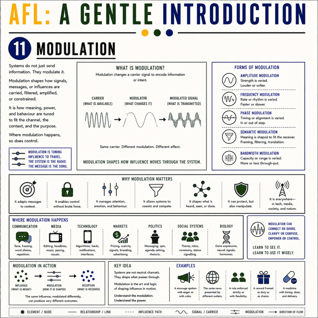
Step 11: Modulation
Once interfaces are identified, intervention becomes a question of modulation.
We write
F′ = M(I(F))
Modulation acts through interfaces rather than directly upon isolated objects.
The practical question therefore changes.
Instead of asking
“What object should we change?”
Applied Field Logic asks
“Which interface should we modulate?”
—
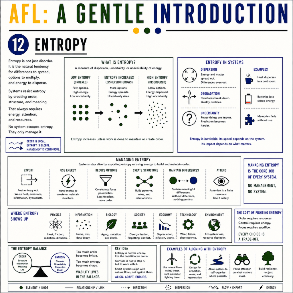
Step 12: Entropy
Entropy is often introduced as disorder.
Applied Field Logic emphasises a relational interpretation.
A familiar expression is
H = −Σ pᵢ log(pᵢ)
Higher entropy corresponds to a broader distribution of possible relational configurations.
Lower entropy corresponds to a narrower range of possible configurations.
This interpretation extends rather than replaces the conventional mathematical treatment.
—
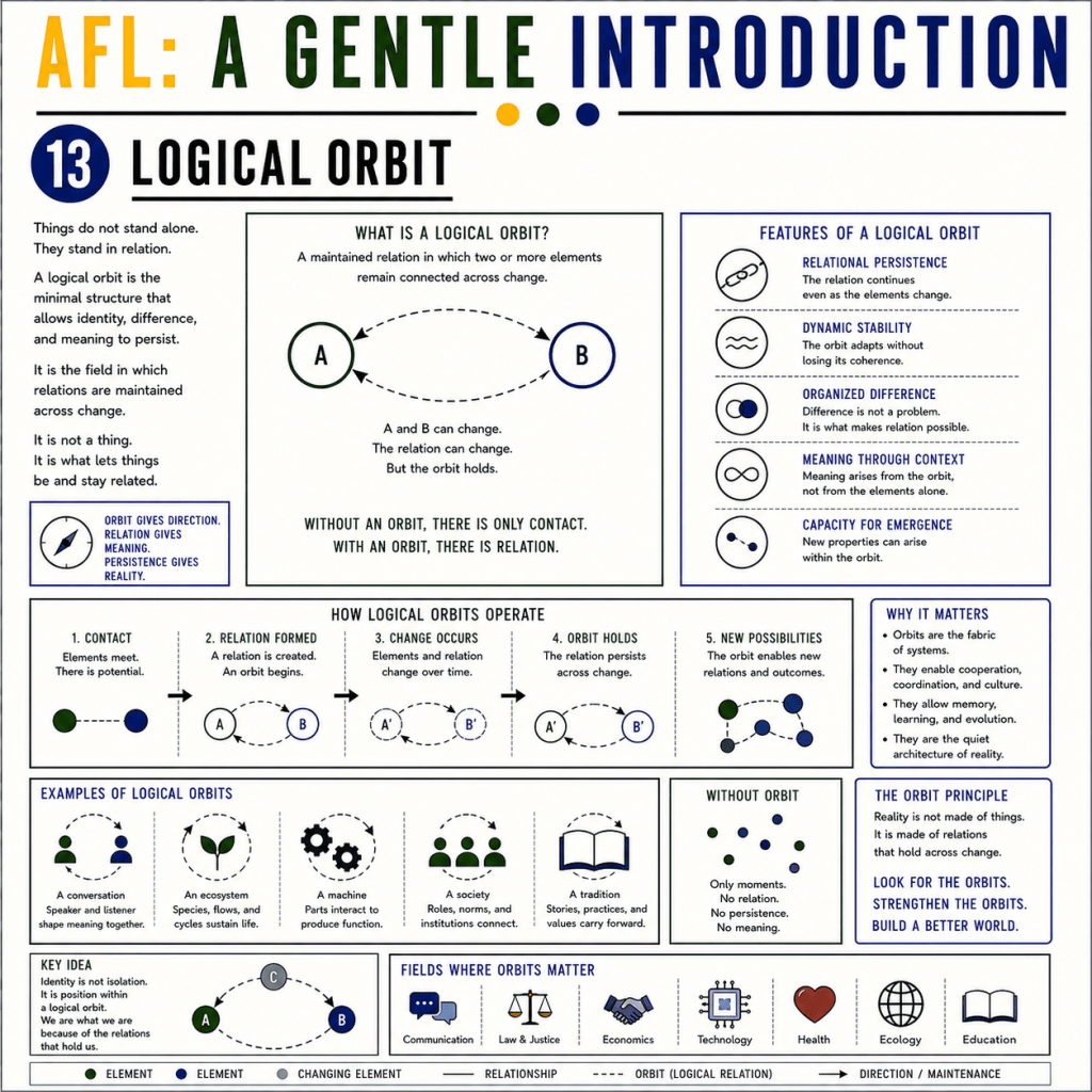
Step 13: The Logical Orbit
We now arrive at the central organising idea.
Objects do not persist independently.
Persistent organisation resides in maintained patterns of relationship.
Applied Field Logic therefore defines the Logical Orbit as
O = (L, H, R(L,H))
where
L is local organisation,
H is the distributed relational horizon,
and
R(L,H) is the maintained relationship between them.
Persistence belongs to the orbit rather than either endpoint alone.
—
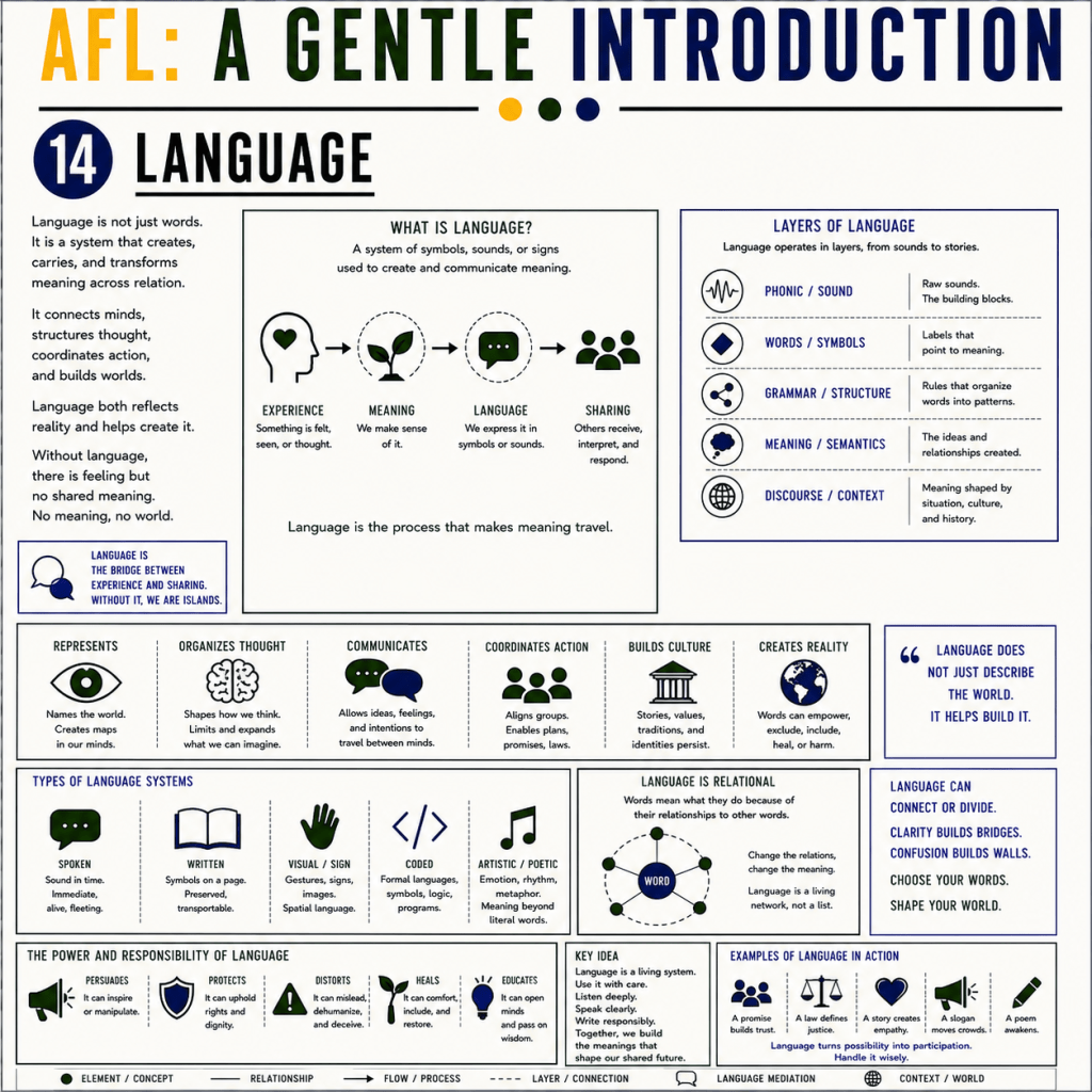
Step 14: Language
Language behaves like every other relational field.
Words do not carry meaning independently.
Meaning emerges through stable patterns of relational use.
We may summarise this schematically as
Meaning = f(Frequency, Coupling)
This expression is conceptual rather than literal.
Repeated relational patterns become stable semantic structures.
Language is therefore understood as a synchronising field rather than merely a collection of symbols.
—
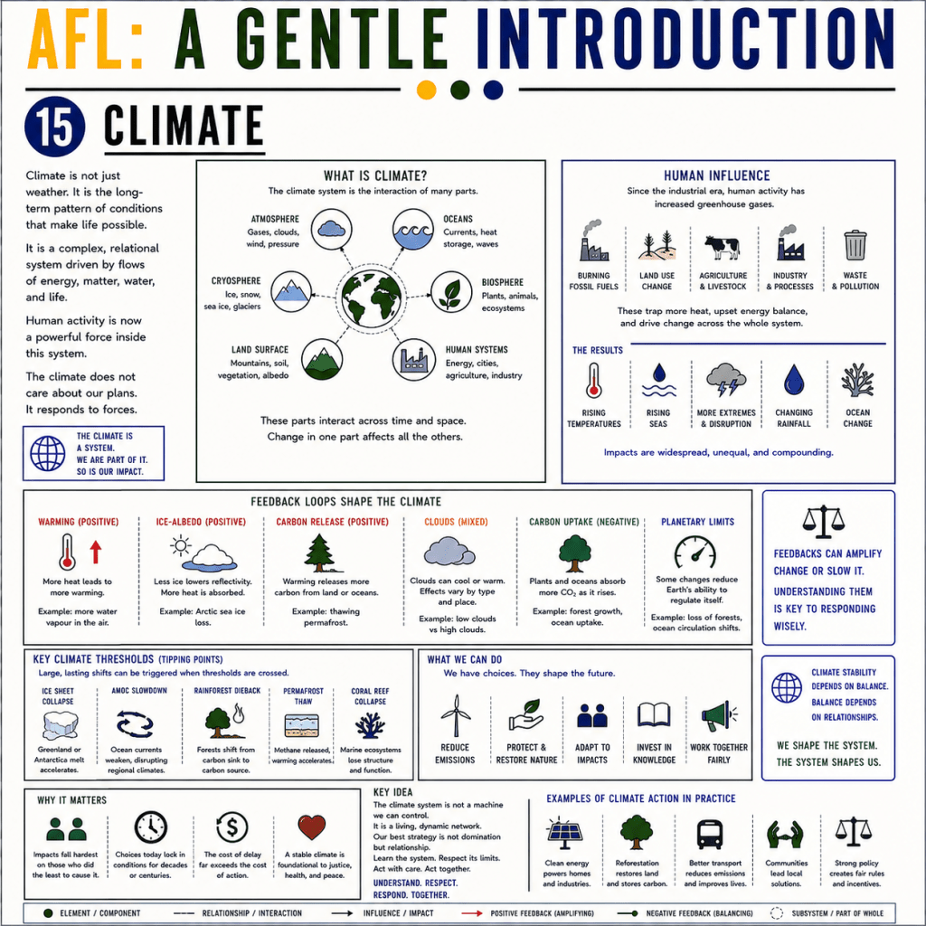
Step 15: Climate
Within this framework, climate is not viewed simply as an environmental system.
It is a planetary relational field.
Atmosphere.
Ocean.
Biology.
Technology.
Economics.
Politics.
Culture.
Language.
These are different interfaces through which one continuous relational organisation becomes observable.
—
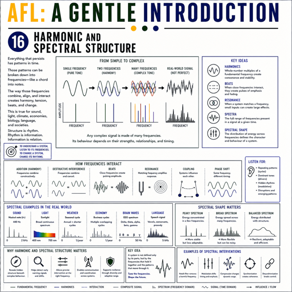
Step 16: Harmonic and Spectral Structure
Real systems contain many rhythms simultaneously.
Daily.
Seasonal.
Economic.
Political.
Ecological.
Technological.
Their interaction produces harmonic structure.
Signal theory shows that repeated behaviour often reveals hidden frequencies.
Applied Field Logic extends this intuition to relational systems.
Heatwaves.
Migration.
Market instability.
Media cycles.
Ecological collapse.
These may all be interpreted as local spectral signatures of deeper organisational dynamics.
—
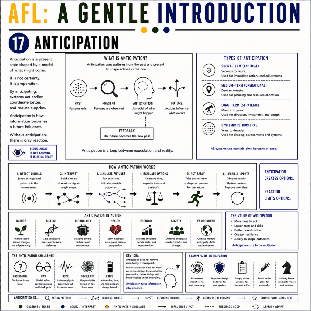
Step 17: Anticipation
Human beings organise themselves around futures that do not yet exist.
Insurance.
Investment.
Planning.
Migration.
Policy.
Present behaviour is therefore shaped by anticipated future states.
Applied Field Logic introduces a formal framework for describing this anticipatory organisation, developed more fully in the mathematical foundations paper.
—
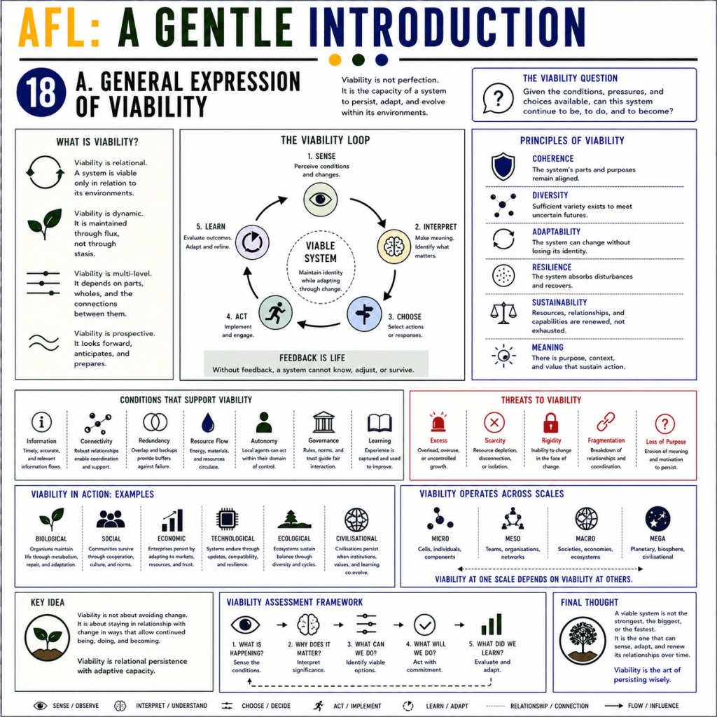
Step 18: A General Expression for Viability
The framework may be summarised schematically as
V(F) = f(P, K, Φ, H, I, S)
where
V = viability
F = relational field
P = persistence
K = coupling
Φ = phase structure
H = entropy
I = interface operators
S = spectral structure
This is not proposed as a universal law of nature.
It is a compact map of the conceptual architecture developed by Applied Field Logic.
—
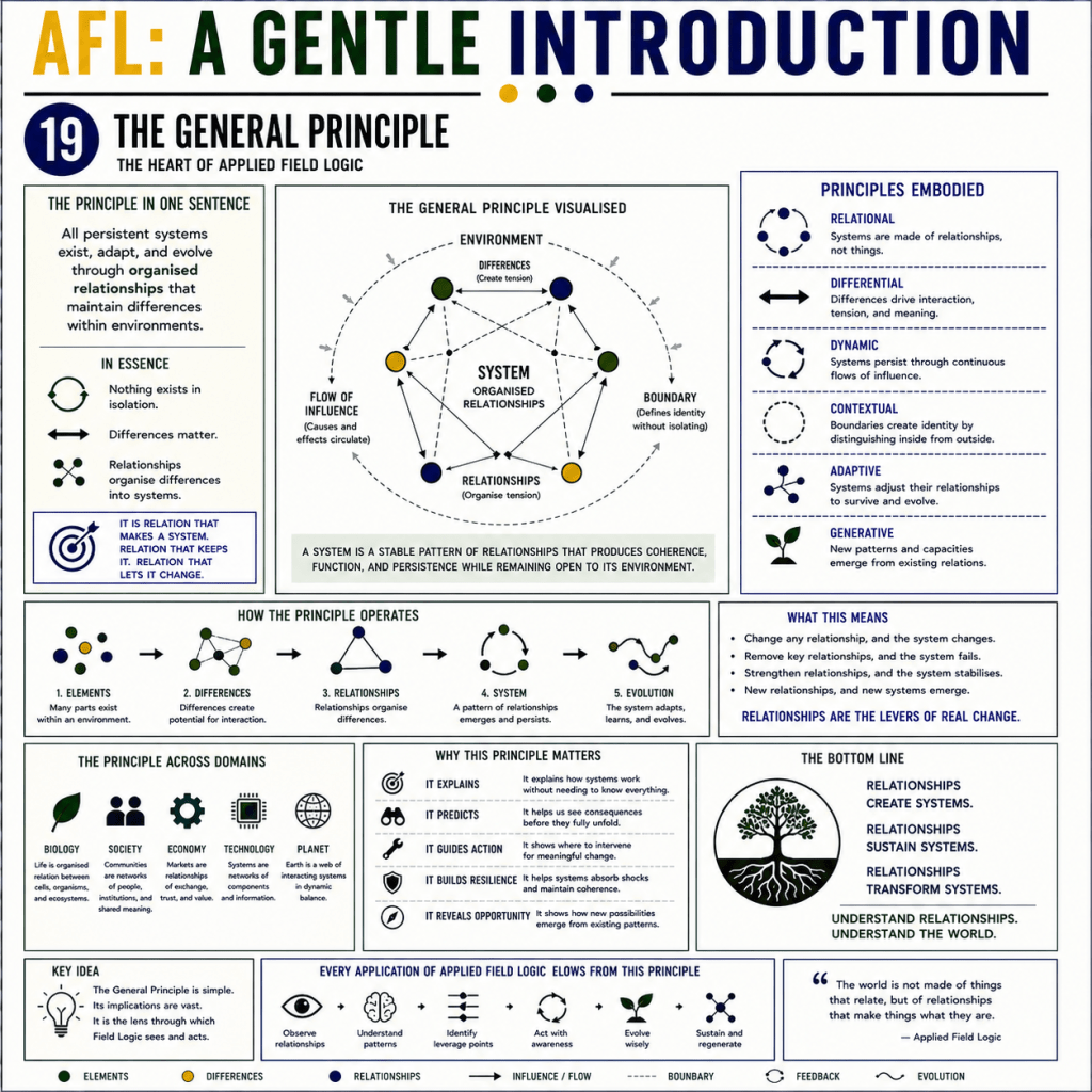
Step 19: The General Principle
Applied Field Logic may be summarised as a single progression.
Distinctions generate differences.
Differences generate relationships.
Relationships generate fields.
Fields generate phase relationships.
Phase relationships generate synchronisation.
Synchronisation generates persistence.
Persistence generates identity.
Identity generates the appearance of stable objects.
Classical thinking begins with objects and derives relationships.
Applied Field Logic begins with relationships and derives the appearance of stable objects.
—
Where Next?
This tutorial introduces only the foundational ideas.
The companion paper, Applied Field Logic: Mathematical Foundations, develops these concepts into a more rigorous framework, including orbit theory, interface calculus, recursive tension, harmonic fields, topological defects, probability landscapes, and spectral semantics.
The mathematics grows from the ontology rather than being imposed upon it.
The equations are not the theory. They are one language through which the theory may be expressed. Its central claim is this:
Persistence, meaning, life, communication, climate, and civilisation emerge from organised relational asymmetry maintained through continuously transforming relational fields.
